Sklearn Decision Tree Unknown Label Type Continuous

In this tutorial, you'll learn how to create a decision tree classifier using Sklearn and Python. Decision trees are an intuitive supervised machine learning algorithm that allows you to classify data with high degrees of accuracy. In this tutorial, you'll learn how the algorithm works, how to choose different parameters for your model, how to test the model's accuracy and tune the model's hyperparameters.

This tutorial assumes no prior knowledge of how decision tree classifier algorithms work. It's intended to be a beginner-friendly resource that also provides in-depth support for people experienced with machine learning.

By the end of this tutorial, you'll have walked through a complete, end-to-end machine learning project. You will have learned:

• How the decision tree classifier algorithm works to predict types of classes
• How the algorithm works with a single dimension and with multiple dimensions
• How to measure the accuracy of your machine learning model
• How to work with categorical and non-numeric data in decision tree classifiers
• How to tweak various hyperparameters of the algorithm to increase the algorithm's accuracy

Let's get started with learning about decision tree classifiers in Scikit-Learn!

• What are Decision Tree Classifiers?
• Why are Decision Tree Classifiers a Good Algorithm to Learn?
• How do Decision Tree Classifiers Work?
• Using Decision Tree Classifiers in Python's Sklearn
• Validating a Decision Tree Classifier Algorithm in Python's Sklearn
• How to Work with Categorical Data in Decision Tree Classifiers
• Do You Need to Scale or Preprocess Data For Decision Tree Classifiers?
• Hyperparameter Tuning for Decision Tree Classifiers in Sklearn
• What to Learn After This Tutorial
• Conclusion
• Additional Resources

What are Decision Tree Classifiers?

Decision tree classifiers are supervised machine learning models. This means that they use prelabelled data in order to train an algorithm that can be used to make a prediction. Decision trees can also be used for regression problems. Much of the information that you'll learn in this tutorial can also be applied to regression problems.

Decision tree classifiers work like flowcharts. Each node of a decision tree represents a decision point that splits into two leaf nodes. Each of these nodes represents the outcome of the decision and each of the decisions can also turn into decision nodes. Eventually, the different decisions will lead to a final classification.

The diagram below demonstrates how decision trees work to make decisions. The top node is called the root node. Each of the decision points are called decision nodes. The final decision point is referred to as a leaf node.

A Sample Decision Tree Visualized

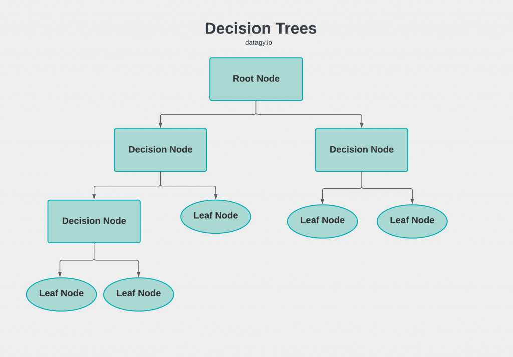
It's easy to see how this decision-making mirrors how we, as people, make decisions!

Why are Decision Tree Classifiers a Good Algorithm to Learn?

Decision trees are a great algorithm to learn for many reasons. One of the main reasons its great for beginners is that it's a "white box" algorithm, meaning that you can actually understand the decision-making of the algorithm. This is especially useful for beginners to understand the "how" of machine learning.

Beyond this, decision trees are great algorithms because:

• They're generally faster to train than other algorithms such as neural networks
• Their complexity is a by-product of the data's attributes and dimensions
• It's a non-parametric method meaning that they do not depend on probability distribution assumptions
• They can handle high dimensional data with high degrees of accuracy

How do Decision Tree Classifiers Work?

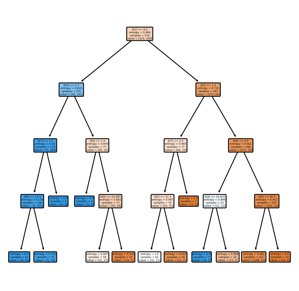
Decision trees work by splitting data into a series of binary decisions. These decisions allow you to traverse down the tree based on these decisions. You continue moving through the decisions until you end at a leaf node, which will return the predicted classification.

The image below shows a decision tree being used to make a classification decision:

A working example of the decision tree you'll build in this tutorial

How does a decision tree algorithm know which decisions to make? The algorithm uses a number of different ways to split the dataset into a series of decisions. One of these ways is the method of measuring Gini Impurity.

Gini Impurity refers to a measurement of the likelihood of incorrect classification of a new instance of a random variable if that instance was randomly classified according to the distribution of class labels from the dataset.

Ok, that sentence was a mouthful! The Gini Impurity measures the likelihood that an item will be misclassified if it's randomly assigned a class based on the data's distribution. To generalize this to a formula, we can write:

The formula for Gini Impurity

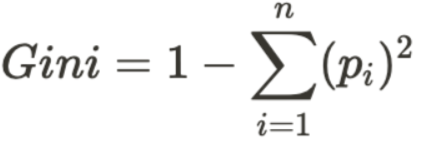
The Gini Impurity is lower bounded to zero, meaning that the closer to zero a value is, the less impure it is.

We can calculate the impurity using this Python function:

          # Calculating Gini Impurity of a Pandas DataFrame Column def gini_impurity(column):     impurity = 1     counters = Counter(column)     for value in column.unique():         impurity -= (counters[value] / len(column)) ** 2      return impurity        

How do we actually put this to use? We split the data by any of the possible values. Let's take a look at an example. Say we are trying to use a decision tree to classify based on a number of different factors, as shown in the image below:

The various attributes that can determine whether someone will exercise or not

In this case, we have three dimensions, 'Weather', 'Ate Breakfast', and 'Slept Enough' to determine our label 'Will Exercise'. In order to figure out what split creates the least impure decision (i.e., the cleanest split), we can run through the same exercise multiple times.

1. We split the data along each unique element
2. We calculate the Gini Impurity for each split of the target value
3. We weight each Gini Impurity based on the overall scores

Let's see what this looks like:

Splitting on whether the weather was Sunny or not

In this example, we split the data based only on the 'Weather' feature. We look first at the outcomes of what the counts for each target are based on this split. We can see that when the weather was sunny, there was an equal split of 2 and 2. When the weather was not sunny, there were two times we didn't exercise and only one time we did.

We then calculate the weighted Gini Impurity for each of these splits. Then, we calculate the weighted value, as shown below:

Calculating weighted impurities

We complete this for each of the possibilities and figure out which returns the lowest weighted impurity. The split that generates the lowest weighted impurity is the one that's used for the split.

Thankfully, sklearn automates this process for you, but it can be helpful to understand why decisions are being made in the way that they are.

In a later section, you'll learn some of the different ways in which these decision nodes are created. This has an important impact on the accuracy of your model.

In the next section, you'll start building a decision tree in Python using Scikit-Learn.

Using Decision Tree Classifiers in Python's Sklearn

Let's get started with using sklearn to build a Decision Tree Classifier. In order to build our decision tree classifier, we'll be using the Titanic dataset. Let's take a few moments to explore how to get the dataset and what data it contains:

          # Downloading an exploring the Titanic dataset import pandas as pd data = pd.read_csv(     'https://github.com/datagy/data/raw/main/titanic.csv',      usecols=['Survived', 'Pclass', 'Sex', 'Age', 'SibSp', 'Fare', 'Embarked']) data = data.dropna()  print(data.head())  # Returns: #    Survived  Pclass     Sex   Age  SibSp  Parch     Fare Embarked # 0         0       3    male  22.0      1      0   7.2500        S # 1         1       1  female  38.0      1      0  71.2833        C # 2         1       3  female  26.0      0      0   7.9250        S # 3         1       1  female  35.0      1      0  53.1000        S # 4         0       3    male  35.0      0      0   8.0500        S        

We dropped any missing records to keep the scope of the tutorial limited. Technically, we could have found ways to impute the missing data, but that's a topic for a broader discussion.

We have a number of features available to us, some of which are numeric and some of which are categorical. Let's take a closer look at these features:

Feature	Description	Data Type
Pclass	The class of the ticket that was purchased	Ordinal
Sex	The sex of the passenger	String / Categorical
Age	The age of the passenger	Float
SibSp	# of siblings / spouses on the Titanic	Integer
Parch	# of parents / children on the Titanic	Integer
Fare	The fare the passenger paid	Float
Embarked	The port where the passenger embarked	C = Cherbourg, Q = Queenstown, S = Southampton

The features of the Titanic dataset

Let's better understand the distribution of the data by plotting a pairplot using Seaborn. We'll temporarily load the target feature into the DataFrame to be able to color points based on whether people survived.

          # Plotting a Pairplot of Titanic Data import pandas as pd import seaborn as sns import matplotlib.pyplot as plt  data = pd.read_csv(     'https://github.com/datagy/data/raw/main/titanic.csv',      usecols=['Survived', 'Pclass', 'Sex', 'Age', 'SibSp', 'Parch', 'Fare', 'Embarked']) data = data.dropna()  sns.pairplot(data=data, hue='Survived') plt.show()        

This returns the following image:

A pairplot of the Titanic Dataset

Based on the image above, we can see that there are a number of clear separations in the data. This can be quite helpful in splitting our data into pure splits using a decision tree classifier.

Before we dive much further, let's first drop a few more variables. In particular, we'll drop all the non-numeric variables for now. Machine learnings tend to require numerical columns to work. We'll focus on these later, but for now we'll keep things simple:

          # Loading only numeric columns import pandas as pd  data = pd.read_csv(     'https://github.com/datagy/data/raw/main/titanic.csv',      usecols=['Survived', 'Pclass', 'Age', 'SibSp', 'Parch', 'Fare']) data = data.dropna()  X = data.copy() y = X.pop('Survived')        

In the code above, we loaded only the numeric columns (by removing 'Sex' and 'Embarked'). Then, we split the data into two variables:

• X: our features matrix (because it's a matrix, it's denoted with a capital letter)
• y: our target variable

We used the .pop() method to create our variable y. This extracts the column and removes it from the original DataFrame.

Now let's first split our data into testing and training data.

Splitting Data into Training and Testing Data in Sklearn

By splitting our dataset into training and testing data, we can reserve some data to verify our model's effectiveness. We do this split before we build our model in order to test the effectiveness against data that our model hasn't yet seen.

We can also split our data into training and testing data to prevent overfitting our analysis and to help evaluate the accuracy of our model. This can be done using thetrain_test_split() function in sklearn. For a further discussion on the importance of training and testing data, check out my in-depth tutorial on how to split training and testing data in Sklearn.

Let's first load the function and then see how we can apply it to our data:

          # Splitting data into training and testing data from sklearn.model_selection import train_test_split  X_train, X_test, y_train, y_test = train_test_split(X, y, random_state = 100)        

In the code above, we:

1. Load the train_test_split function
2. We then create four variables for our training and testing data
3. We assign the random_state= parameter here to ensure that we have reproducible results

Now that we have our data split in a meaningful way, let's explore how we can use the DecisionTreeClassifier in Sklearn.

Understanding DecisionTreeClassifier in Sklearn

In this section, we'll explore how the DecisionTreeClassifier class works in Sklearn. We can import the class from the tree module. Let's see how we can import the class and explore its different parameters:

          # How to Import the DecisionTreeClassifer Class from sklearn.tree import DecisionTreeClassifier DecisionTreeClassifier(     *,      criterion='gini',      splitter='best',      max_depth=None,      min_samples_split=2,      min_samples_leaf=1,      min_weight_fraction_leaf=0.0,      max_features=None,      random_state=None,      max_leaf_nodes=None,      min_impurity_decrease=0.0,      class_weight=None,      ccp_alpha=0.0 )        

Let's take a closer look at these parameters:

Parameter	Default Value	Description
criterion=	'gini'	The function to measure the quality of a split. Either 'gini' or 'entropy'.
splitter=	'best'	The strategy to choose the best split. Either 'best' or 'random'
max_depth=	None	The maximum depth of the tree. If None, the nodes are expanded until all leaves are pure or until they contain less than the min_samples_split
min_samples_split=	2	The minimum number of samples required to split a node.
min_samples_leaf=	1	The minimum number of samples require to be at a leaf node.
min_weight_fraction_leaf=	0.0	The minimum weighted fraction of the sum of weights of all the input samples required to be at a node.
max_features=	None	The number of features to consider when looking for the best split. Can be: – int, – float, – 'auto' (the square root of number of features), – 'sqrt' (same as auto), – 'log2' (log of number of features), – None (the number of features)
random_state=	None	The control for the randomness of the estimator
max_leaf_nodes=	None	Grow a tree with a maximum number of nodes. If None, then an unlimited number is possible.
min_impurity_decrease=	0.0	A node will be split if this split decreases the impurity greater than or equal to this value.
class_weight=	None	Weights associated with different classes.
ccp_alpha=	0.0	Complexity parameter used for Minimal Cost-Complexity Pruning.

The parameters available in the DecisionTreeClassifier class in Sklearn

In this tutorial, we'll focus on the following parameters to keep the scope of it contained:

• criterion
• max_depth
• max_features
• splitter

One of the great things about Sklearn is the ability to abstract a lot of the complexity behind building models. Because of this, we can actually create a Decision Tree without making any decisions ourselves. We can do this, by using the default parameters provided by the class.

Now, let's see how we can build our first decision tree classifier using Sklearn!

          # Creating Our First Decision Tree Classifier from sklearn.tree import DecisionTreeClassifier clf = DecisionTreeClassifier() clf.fit(X_train, y_train)        

In the code above we accomplished two critical things (in very few lines of code):

1. We created our Decision Tree Classifier model and assigned it to the variable clf
2. We then applied the .fit() method to train the model. In order to do this, we passed in our training data.

Scikit-Learn takes care of making all the decisions for us (for better or worse!). Now, let's see how we can make predictions with this newly created model:

          # Making Predictions with Our Model predictions = clf.predict(X_test) print(predictions[:5])        

Let's break down what we did in the code above:

1. We assigned a new variable, predictions, which takes the values from applying the .predict() method to our model clf.
2. We make predictions based on our X_test data

When we printed out the first five records of our predicted values, where 0 represents that a passenger did not survive, while a 1 indicates that they did survive.

How do we know how well our model is performing? That's something that we'll discuss in the next section!

Validating a Decision Tree Classifier Algorithm in Python's Sklearn

Different types of machine learning models rely on different accuracy metrics. When we made predictions using theX_test array, sklearn returned an array of predictions. We already know the true values for these: they're stored iny_test.

We can use the sklearn function,accuracy_score() to return a proportion out of 1 that measures the algorithms effectiveness. The accuracy score looks at the proportion of accurate predictions out of the total of all predictions.

Let's see how we can do this:

          # Measuring the accuracy of our model from sklearn.metrics import accuracy_score print(accuracy_score(y_test, predictions))  # Returns: 0.6815642458100558        

We can see that the accuracy score that's returned is 0.68, or 68%. This means that for all of the values we attempted to predict, 68% of them were correct.

One of the ways in which we can attempt to improve the accuracy of a model is by adding in more useful features. Previously, we omitted non-numerical data. Let's see how we can include them in our model.

How to Work with Categorical Data in Decision Tree Classifiers

Machine learning models require numerical data to work. When passing in non-numeric data, the model building process fails. Let's take a look at how this looks. We'll load in the columns of 'Sex' and 'Embarked' and see if we can build our model:

          # Attempting to build a model with non-numeric data import pandas as pd from sklearn.model_selection import train_test_split from sklearn.tree import DecisionTreeClassifier from sklearn.metrics import accuracy_score  X = pd.read_csv(     'https://github.com/datagy/data/raw/main/titanic.csv',      usecols=['Survived', 'Pclass', 'Age', 'SibSp', 'Parch', 'Fare', 'Sex', 'Embarked']) X = X.dropna() y = X.pop('Survived')  X_train, X_test, y_train, y_test = train_test_split(X, y, random_state = 100)  clf = DecisionTreeClassifier() clf.fit(X_train, y_train)  # Raises # ValueError: could not convert string to float: 'female'        

Does this mean that we're stuck? No – we simply need to find a way to convert our non-numeric data into numeric data. One way to do this is to use a process known as one-hot encoding.

One-hot encoding converts all unique values in a categorical column into their own columns. The column is then assigned the value of 1 if the column matches the original value, and 0 otherwise. The image below breaks this down:

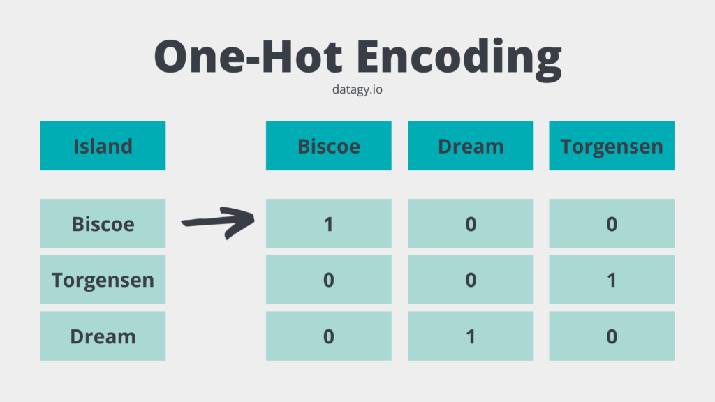
You may be wondering why we didn't encode the data as 0, 1, and 2. The reason for this is that the data isn't ordinal or interval data, where the order means anything. Assigning a value of 0 to one value and 2 to another would imply the difference between these two values is greater than between one value and another.

By doing this, we can safely use non-numeric columns. Let's see how we can use Python and Scikit-Learn to convert our columns to their one-hot encoded columns.

          # One-hot encoding our data from sklearn.preprocessing import OneHotEncoder from sklearn.compose import make_column_transformer  column_transformer = make_column_transformer(     (OneHotEncoder(), ['Sex', 'Embarked']),     remainder='passthrough')  X_train = column_transformer.fit_transform(X_train) X_train = pd.DataFrame(data=X_train, columns=column_transformer.get_feature_names())        

Let's break down what we did here:

1. We imported the OneHotEncoder() class and the make_column_transformer function
2. We created a column transformer object
3. We then apply the .fit_transform() method to simultaneously fit and transform the column transformations on the X_train dataset
4. We then converted the dataset back into a Pandas DataFrame

Let's see how we can now use our dataset to make classifications using a Decision Tree Classifier in Scikit-Learn:

          # Making Predictions with One-Hot Encoded Values X_test = column_transformer.transform(X_test) X_test = pd.DataFrame(data=X_test, columns=column_transformer.get_feature_names())  clf = DecisionTreeClassifier() clf.fit(X_train, y_train)  predictions = clf.predict(X_test) print(accuracy_score(y_test, predictions))  # Returns: 0.775        

Let's break down what we did here:

1. We one-hot encoded out X_test variable. Note here, that we only applied the .transform() method in order to one-hot encode our testing data.
2. We then created our model and fitted it using the training data.
3. Finally, we made predictions using the .predict() method and checked its accuracy.

In this case, we were able to increase our accuracy to 77.5%!

Do You Need to Scale or Preprocess Data For Decision Tree Classifiers?

Many machine learning algorithms are based on distance calculations. In our earlier discussions about impurity and entropy, we learned that this isn't true for decision trees.

Because of this, scaling or normalizing data isn't required for decision tree algorithms. This can save us a bit of time when creating our model.

Hyperparameter Tuning for Decision Tree Classifiers in Sklearn

To close out this tutorial, let's take a look at how we can improve our model's accuracy by tuning some of its hyper-parameters. Hyper-parameters are the variables that you specify while building a machine learning model. This includes, for example, how the algorithm splits the data (either by entropy or gini impurity).

Hyper-parameter tuning, then, refers to the process of tuning these values to ensure a higher accuracy score.One way to do this is, simply, to plug in different values and see which hyper-parameters return the highest score.

Rather than trying out a whole slew of different combinations, Scikit-learn provides a way to automate these tests. This method is the GridSearchCV method, which makes the process significantly faster. We simply need to provide a dictionary of different values to try and Scikit-Learn will handle the process for us.

Furthermore, the class completes a process of cross-validation. This means that the class will cycle through different combinations of training and testing data, in order to help prevent overfitting. For example, when we set a test size of 20%, cross-validation will cycle through different splits of that 20% in relation to the whole.

Let's see what this looks like visually:

Visualizing how Cross-Validation Works in Machine Learning

Let's see how we can apply the GridSearchCV class to both find the best hyperparameters and apply cross-validation at the same time.

In order to do this, we first need to decide which hyperparameters to test. Let's see which ones we will be using:

• criterion – the function that's used to determine the quality of a split
• max_depth – the maximum depth of the tree
• max_features – the max number of features to consider when making a split
• splitter – the strategy used to choose the split at each node

Let's see how we can make this work:

          # Creating a dictionary of parameters to use in GridSearchCV from sklearn.model_selection import GridSearchCV  params = {     'criterion':  ['gini', 'entropy'],     'max_depth':  [None, 2, 4, 6, 8, 10],     'max_features': [None, 'sqrt', 'log2', 0.2, 0.4, 0.6, 0.8],     'splitter': ['best', 'random'] }  clf = GridSearchCV(     estimator=DecisionTreeClassifier(),     param_grid=params,     cv=5,     n_jobs=5,     verbose=1, )  clf.fit(X_train, y_train) print(clf.best_params_)        

This returns the following dictionary:

          # The best parameters {     'criterion': 'entropy',      'max_depth': 4,      'max_features': 0.6,      'splitter': 'best' }        

Keep in mind, that even though these parameters are labeled as the best parameters, this is in the context of the parameter combinations that we passed in. There could, theoretically, be better parameters.

Let's now recreate and evaluate our model and see what the score is now:

          # Using the Parameters from GridSearchCV import pandas as pd from sklearn.model_selection import train_test_split from sklearn.tree import DecisionTreeClassifier from sklearn.metrics import accuracy_score  X = pd.read_csv(     'https://github.com/datagy/data/raw/main/titanic.csv',      usecols=['Survived', 'Pclass', 'Age', 'SibSp', 'Parch', 'Fare', 'Sex', 'Embarked']) X = X.dropna() y = X.pop('Survived')  from sklearn.preprocessing import OneHotEncoder from sklearn.compose import make_column_transformer  X_train, X_test, y_train, y_test = train_test_split(X, y, random_state = 100)  column_transformer = make_column_transformer(     (OneHotEncoder(), ['Sex', 'Embarked']),     remainder='passthrough')  X_train = column_transformer.fit_transform(X_train) X_train = pd.DataFrame(data=X_train, columns=column_transformer.get_feature_names())  X_test = column_transformer.transform(X_test) X_test = pd.DataFrame(data=X_test, columns=column_transformer.get_feature_names())  clf = DecisionTreeClassifier(max_depth=4, criterion='entropy', max_features=0.6, splitter='best') clf.fit(X_train, y_train) predictions = clf.predict(X_test)  print(accuracy_score(y_test, predictions))  # Returns: 0.812        

The code block above includes the entirety of the code, where our model returned an accuracy of over 80%!

What to Learn After This Tutorial

Phew! You've made it to the end! At this point, you may be wondering where to go next. The best next step is to work with some of your own data and see how you can apply what you've learned. Try and learn about some of the other hyperparameters available in the Decision Tree classifier.

Following that, I suggest looking at this tutorial covering random forests. Decision trees can be prone to overfitting and random forests attempt to solve this. These build on decision trees and leverage them to prevent overfitting. Check out my tutorial on random forests to learn more.

Conclusion

In this tutorial, you learned all about decision tree classifiers in Python. You learned what decision trees are, their motivations, and how they're used to make decisions. Then, you learned how decisions are made in decision trees, using gini impurity.

Following that, you walked through an example of how to create decision trees using Scikit-Learn. You learned how the algorithm is used to work with numeric and non-numeric data. You also learned how to assess the accuracy of your algorithm and how to improve it using grid search and cross-validation.

Additional Resources

To learn more about related topics, check out the tutorials below:

• Introduction to Scikit-Learn (sklearn) in Python
• Linear Regression in Scikit-Learn (sklearn): An Introduction
• Introduction to Random Forests in Scikit-Learn (sklearn)
• Support Vector Machines (SVM) in Python with Sklearn
• K-Nearest Neighbor (KNN) Algorithm in Python
• Official Documentation: Decision Tree Classifier

giannonesamelle1983.blogspot.com

Source: https://datagy.io/sklearn-decision-tree-classifier/

Share this post